
Making memory bound kernels go brr on a MI300X
A not-so brief recap of an attempt to mess around with memory bound kernels to make 'em faster, and learn something along the adventure.

Kernels, kernels, kernels. They come in a variety of flavors that unusually depend on what the Boy Scout selling popcorn (as a former Boy Scout, highly recommend!) at your door has in stock. Caramel, chocolate, and so on. Yum yum yum. But I’m not talking about this kernel

I’m referring to this one.

My day-to-day activities have compelled me to delve deeper into kernels programmed via HIP (ROCm’s equivalent of the CUDA programming language). And just like popcorn, we can say that GPU kernels have different flavors. I’ll opt to flavorize them purely based on arithmetic intensity, which is traditionally defined as the ratio between floating point operations (FLOP) and bytes loaded by a GPU kernel. From there, we can find the ridge point of the MI300X after a couple of quick datasheet lookups.
The peak memory bandwidth is 5.3 TB/s
The maximum compute in single point floating precision (FP32) that we can do is 163.4 TFLOPs
Using these numbers, the derived ridge point value is:
In this blog, we’ll go through and try to understand how we can speed up a vector add with a simple ROCM tweak — cache bypassing — to make our kernels approach theoretical maximum performance set out by our hardware’s physical limitations. The role of a performance engineer with respect to kernels is always to try and see how close we can get to achieving complete utilization of the hardware.
Let’s play around with a vector add kernel. In short, here’s the starting kernel implementation:
__global__ void vectorAdd(const float* A, const float* B, float* C, int n) {
    int idx = blockIdx.x * blockDim.x + threadIdx.x;
    if (idx < n) {
        C[idx] = A[idx] + B[idx];
    }
}
And a roofline to get an idea of perf.

In the memory bound regime, our FLOPs are bound by how fast our memory subsystem can fetch data. Unfortunately, we often do NOT get the full 5.3 TB/s that AMD lists on their data sheet in practice, so our performance is worse than the latency you’d expect purely from loading data (I’m making the “roofline assumption” that our kernel runtime can be approximated as the max of either purely memory, and compute; memory in this case).
So, we’ll define a figure of merit (FoM). Our job as performance engineers is to milk the most performance we can out of our system, and in this case, we’ll say that can be done by maximizing our bandwidth utilization, which is the ratio of the bandwidth our hardware performance counters report to the theoretical bandwidth AMD lists for the MI300X — 5.3 TB/s.
By doing this with a simple vector add kernel, we’ll garner some intuition on memory bound kernels that we can apply to more complex kernels (not touched upon in this blog).
Table of Contents:
Overview of the MI300X’s Memory Subsystem
Top Level Chiplet Organization
Cache Hierarchy, and (what we know on) cache configurations
Building intuition on what the GPU ends up doing in the workload
Connecting performance counters & AMD data back to the hardware
Examining performance counter changes pre-and post optimization
Asking some questions, and speculating on hardware results.
(Brief) Conclusion
MI300X Memory Subsystem Overview
Unlike the H100 chip, the AMD’s MI300 series of graphics processing units (GPUs) follow the paradigm of chiplet based architectures. In a nutshell, we create small, module units of chips that can be easily pieced together to add more FLOPs or memory bandwidth to the system. In AMD’s terminology, we have two types of chiplets: a compute chiplet referred to as an Accelerator Complex Die (XCD), and an IO chiplet called IOD.
Some things to note about the two
Each XCD contains 40 Compute Units (CU)s. Due to yield constraints, only 38 of these end up working. Think of CUs as being analogous to NVIDIA’s Streaming Multiprocessor in functionality.
Each IOD — designed in tandem with memory manufacturers SK Hynix and Samsung — contain two stacks of High Bandwidth Memory (HBM3) memory. This will become a lot more relevant to us, as AMD leverages an interface called the External Arbiter (EA) that connects the final L2 Cache (L2C) with the fabric Last Level Cache (LLC), aka the InfinityCache, which then interfaces with the IOD via a silicon interposer.

For now, assume that all caches are on the compute chiplet XCD, and that memory is on IOD. Hopefully that gets us to a working picture of the hardware model. A critical part of what we’ll need to look at for our optimizations is the cache hierarchy of the memory subsystem.

Data from registers moves out in a straightforward path, going through each level of the cache until it eventually percolates up to HBM.
The L1C - aka vL1D / Text Cache Pipe (TC) - is the first layer of temporary storage. With CDNA 3, which refers to the specification for XCDs, the vector L1 Data Cache (vL1D) supports 128-byte cache lines, and has a capacity of 32 KB. Similarly, there is a 16 KB scalar L1 Data Cache, which is exclusively used for memory operations (ops) that involve loading single elements over coalesced memory vector ops. Both of these are per-CU.
At the same level of the L1C is the 64 KB software controlled Local Data Store (LDS), also per CU. The LDS uses scratchpad SRAM memory, so it’s slower than registers, but still eons faster than the 5.3 TB/s HBM DRAM we use.
Next level, we get to the L2C - aka Texture Cache Channel (TCC) -, which is per XCD. That means it’s shared across all 38 (2 of the 40 CUs are expected to be powered off or failing from fabrication) CUs. The L2 is a 4 MB write-back cache.
Finally, our L3C / LLC is 256 MB, and notably is on the IOD instead of the XCD, unlike our previous caching hierarchies. It is allegedly a 16-way set associative cache, with there being 128 slices of 2 MB each.
As a side point, coherency, or the process of making sure that everyone has the same copy of data, is handled at the L2C level via a directory based cache coherency protocol. We end up needing pretty sophisticated coherence mechanisms considering that our GPU is effectively 8 private “mini GPUs” (XCDs) that each do their own thing, and only share data when they need to.
As a final point, here’s a brief way to think about the optimization we’ll be doing. We can see our average memory access time (AMAT) as an expected value calculation of hitting each of the levels:
But what if we disable caching entirely? Then, our computation simplifies to this.
And the value add here is that passing through each of the caching structures is a lot quicker than accessing it and failing to retrieve data (i.e, a cache miss). So if our caches are failing most of the time, it’s better to just tell the hardware to avoid using them.
The math behind what the GPU ends up doing in the workload
What is our GPU actually processing? Let’s do some minor computations to illustrate the nature of our workload. First, a quick recap of GPUs.
GPUs don’t process things one after another. They’re designed to do loads of work in parallel, overlapping computation by doing so. These computations are done in waves if there’s more things to compute than hardware available.
Now, let’s create a scenario — say, we wish to run this program here.
// vector_add.hip
#include <hip/hip_runtime.h>
#include <iostream>
#include <chrono>

#define N (32 * 1024 * 1024)  // 32M elements
#define THREADS_PER_BLOCK 256

__global__ void vectorAdd(const float* A, const float* B, float* C, int n) {
    int idx = blockIdx.x * blockDim.x + threadIdx.x;
    if (idx < n) {
        C[idx] = A[idx] + B[idx];
    }
}

int main() {
    size_t bytes = N * sizeof(float);

    // Allocate host memory
    float *h_A = new float[N];
    float *h_B = new float[N];
    float *h_C = new float[N];

    // Initialize input vectors
    for (int i = 0; i < N; i++) {
        h_A[i] = 1.0f;
        h_B[i] = 2.0f;
    }

    // Allocate device memory
    float *d_A, *d_B, *d_C;
    hipMalloc(&d_A, bytes);
    hipMalloc(&d_B, bytes);
    hipMalloc(&d_C, bytes);

    // Copy data to device
    hipMemcpy(d_A, h_A, bytes, hipMemcpyHostToDevice);
    hipMemcpy(d_B, h_B, bytes, hipMemcpyHostToDevice);

    // Launch kernel
    int numBlocks = (N + THREADS_PER_BLOCK - 1) / THREADS_PER_BLOCK;

    // Timed execution
    auto start = std::chrono::high_resolution_clock::now();
    hipLaunchKernelGGL(vectorAdd, dim3(numBlocks), dim3(THREADS_PER_BLOCK), 0, 0,
                       d_A, d_B, d_C, N);
    hipDeviceSynchronize();
    auto end = std::chrono::high_resolution_clock::now();

    std::chrono::duration<double> elapsed = end - start;

    // Calculate bandwidth
    double bytesTransferred = 3.0 * bytes; // 2 reads + 1 write
    double bandwidth = bytesTransferred / elapsed.count() / 1e9;

    std::cout << "Execution time: " << elapsed.count() * 1000 << " ms\n";
    std::cout << "Effective bandwidth: " << bandwidth << " GB/s\n";

    // Copy result back
    hipMemcpy(h_C, d_C, bytes, hipMemcpyDeviceToHost);

    // Verify result
    bool correct = true;
    for (int i = 0; i < N; i++) {
        if (fabs(h_C[i] - 3.0f) > 1e-5) {
            correct = false;
            break;
        }
    }
    std::cout << "Result: " << (correct ? "PASSED" : "FAILED") << "\n";

    // Cleanup
    hipFree(d_A);
    hipFree(d_B);
    hipFree(d_C);
    delete[] h_A;
    delete[] h_B;
    delete[] h_C;

    return 0;
}
Here, we have a single kernel that does a vector add across 32 * 1024 * 1024 = 225 = 33,554,432 elements. As we use FP32 precision, each array takes 134,217,728 bytes to hold in memory.
Since we load A, load B, and then store C, we do 3 memory transfers, meaning that our total memory traffic is at least 402,653,184 bytes.
On the other hand, we only do 1 floating point operation — the add — per element. So, we do a total of 134,217,728 floating point operations in this program.
Generally speaking, we have 3 memory transfers for each floating point operation. That means our arithmetic intensity is:
Regardless of the number of elements, our arithmetic intensity shall remain fixed. And it’s wayy less than the 30.83 ridge-point AI* that we calculated prior to this, just telling us how hopelessly memory bound this task is. And the vector-add problem here will remain memory bound regardless of the value for which we set N to be.
Additionally, we define NUM_THREADS = 256 in this situation. In total, that means we have 256 threads per thread block / workgroup. CDNA 3 caps the maximum number of threads per compute unit (CU) at 1024 threads / CU. That means that we will have at most 4 thread blocks per CU.
Our workload requires N / 256 = 217 thread blocks, and as we have at most 4 threadblocks per CU, we need 215 CUs. Per pass, we have 304 CUs. That means we approximately require ceil(215/304) = 108 waves to process the entire workload.
So, this isn’t a “quickie”. There’s a large number of waves, and all compute units would need to be mobilized and utilized for the fastest results.
What do AMD perf counters give us?
To run this tools, I use v2 of AMD’s rocprof utility. It’s an amazing, nifty tool that can be thought of as similar in functionality to ncu for those more familiar with NVIDIA terminology.
Now, we can try to use the metrics that the rocprof tool provides for our MI300X architecture, known to the software as gfx942. First, let’s think about how we can quantify our figure of merit.
Effectively, bandwidth represents the rate at which bytes are read and written. We know the total number of bytes read + written is 402,653,184, and we can query and divide the bytes value by the total runtime of the kernel to get a lower bound to the actual bandwidth.
Here’s what the parsed profiler output tells us:
================================================================================
  GLOBAL MEMORY (HBM/DRAM) ANALYSIS
================================================================================

Total Memory Traffic (Including Cache Effects):
  Data Read (Fetch):............................  262201.62 KB
  Data Written:.................................  131072.00 KB
  Total Traffic:................................  393273.62 KB

Achieved Bandwidth:
  From FETCH/WRITE_SIZE:........................    3807.83 GB/s
  Bandwidth Efficiency:.........................      71.85%
Not too shabby for a vector add. A bandwidth efficiency (i.e, utilization, our FoM) of 71% tells us that the program is already making good use of the memory subsystem. This is critical in our memory bound cases, and something we can improve. It’s also good to see some patterns in the memory traffic — the read traffic is 2x higher as we need to read A and B, and only write C. If we say, divide 134,217,728 by 1000 to convert to KB, we see that 134,217 KB is close to the total data written. That’s a good sign, telling us that perf counters are giving us sensible data.
Let’s move to the L1C, specifically:
================================================================================
  L1 CACHE ANALYSIS
================================================================================

--- Instruction Cache (L1i) ----------------------------------------------------
  Hit Rate:.....................................  99.87%
  ✓ Good instruction cache performance

--- Scalar L1 Data Cache (sL1d) - Uniform/Constant Data ------------------------
  Hit Rate:.....................................  99.76%
  Access Pattern:............................... Uniform (same address for all threads)

--- Vector L1 Data Cache (vL1d/TCP) - Per-Thread Data --------------------------
  Hit Rate (TCB):...............................  87.18%
  Cache Utilization:............................  96.93%
  Buffer Coalescing Rate:....................... 100.00%

L1 Vector Cache Traffic:
  Read Accesses:................................ 16777216
  Write Accesses:............................... 8388608
  Atomic (with return):......................... 0
  Atomic (without return):...................... 0

--- L1 Tag Conflicts (Concurrent Access Stalls) --------------------------------
  Read Tag Conflict Stall:......................   0.00%
  Write Tag Conflict Stall:.....................   0.00%
  Atomic Tag Conflict Stall:....................   0.00%
An L1C hit rate of 99% is great, but not unusual. Typically, caches are somewhat speculative, and may incorporate predictors that help bring that hit rate percentage into the high 90’s.
We do see a lower hit rate in the vL1d cache, which is interesting. Not too sure why that’s happening, but it is a good sign to see a 100% coalescing rate. As 225 is a multiple of our 28 thread size, high wavefront / warp coalescing does make sense, and is what we hope for.
Let’s take a quick glance over at the wave time breakdown. This is more of a compute side perf counter glance, but I do want to provide some data-based validation for why we can apply the roofline assumption in this case.
================================================================================
  WAVEFRONT EXECUTION ANALYSIS
================================================================================

--- Per-Wavefront Metrics ------------------------------------------------------
  Average Wave Duration:........................ 3085.40 cycles
  Total Wave-Cycles (×4):....................... 404410192 quad-cycles
                                                 1617640768 actual cycles

Wave Time Breakdown:
  Executing Instructions:.......................   2.59%
  Waiting on Dependencies:......................  96.03%
  Waiting to Issue:.............................   1.45%
  Total Wait Cycles (×4):....................... 399205137 quad-cycles

--- Thread Divergence Analysis -------------------------------------------------
  Waves with 64 threads active:................. 524288 (100.0%)
  Waves with <64 threads:...................... 0 (0.0%)
  Waves with <48 threads:...................... 0 (0.0%)
  Waves with <32 threads:...................... 0 (0.0%)
  Waves with <16 threads:...................... 0 (0.0%)

  Average Active Threads per Wave:.............. 64.00 / 64
  Thread Utilization:........................... 100.00%
  ✓ Good thread utilization
See the wave time breakdown? The largest time box in this case tells us that we’re spending the majority of our time waiting to fetch dependencies. But our kernel has no data dependencies beyond loading from memory! So, we conclude that we’re constantly waiting on the memory subsystem rather than doing actual computations.
This isn’t something we can do that much about; it just validates our roofline hypothesis that we’re so heavily bound by memory. In general, this is a great example of why roofline analysis works — we see a heavy, 90%+ skew towards waiting on memory, which means we can simply approximate our time by saying our kernel’s actual runtime time is well approximated from just fetching data from memory.
Now, my initial motivation for the optimization itself. L2 data.
================================================================================
  L2 CACHE (TCC) ANALYSIS
================================================================================

L2 Cache Hit Rates:
  Hit Rate (reported):.........................   25.05%
  Hit Rate (calculated):........................  25.05%
  Cache Hits:................................... 1051688
  Cache Misses:................................. 3146122
  Total Accesses:............................... 4197810

L2 Cache Traffic:
  Read Requests:................................ 2100658
  Write Requests:............................... 2097152
  Atomic Requests:.............................. 0

L2 Request Types by Caching Mode:
  Non-Coherent (NC):............................ 0
  Uncached (UC):................................ 298
  Coherent Cached (CC):......................... 0
  Read-Write (RW):.............................. 0

L2 Cache Evictions:
  Writebacks to DRAM:........................... 1048696
  Cache Line Evictions:......................... 3014704

L2 EA Uncached Traffic:
  Uncached Reads  (32B):........................ 598
  Uncached Writes (32B):........................ 0

L2 Pipeline Stalls:
  Tag Pipeline Stall:...........................   0.00%
  Tag RAM Stall Rate:...........................   0.00%
My vibe coded script’s warning gives it away. Our L2 hit rate is terrible. At the time I was messing around, I didn’t have L2 request type stats. So, I didn’t know that the requests were all uncached. But the dismal L2 hit rate of 0.25 tells us that 100-25% = 75% percent of the time, we’re needing to go through the IO dies. So, why not try and disable L2 caching entirely?
Brief primer on caches. Caches are designed with the hope of capturing “spatio temporal locality”. That’s fancy talk for saying if you repeatedly request the same data, or data close to it index-wise in an array, we can store the data each time close by on the XCD compute die instead of taking an eternity crossing chiplets and heading to the HBM stack in IOD. It’s a time tested application of the principle of “reuse where you can”. Specifically, spatio temporal locality can be broken into:
Spatial Locality: Do we access addresses that are nearby?
Temporal Locality: Do we repeatedly reuse an address?
In our program, we do have a good bit of spatial locality as threads access consecutive indices which are hopefully stored in memory. Let’s think about the sequence of accesses and how they walk up the memory hierarchy:
First we try to access data for A[0] and B[0]. L1C, L2C, and LLC do not have this data, leading to cache misses as the memory system scrambles to fetch the data. The L2C stores data in 128-byte cache lines. So, we would retrieve 2 lines (in a simple situation) — 128 bytes of data for A, and 128 bytes for B**. Since we require 4 bytes per float, we literally fetch 128 / 4 = 32 elements of A, and 32 elements of B.
So, we’ve fetched 32 elements for both A and B. But that’s not enough for even a wavefront (warp) in AMD, which has 64 threads each making a request. At this point, we’ve only gotten the data for threads 0 - thread 31. So we’ll need to fetch another line for A and another for B to satisfy the full wavefront.Remember the buffer coalescing rate being 100%? That’s critical for performance. AMD caps the number of threads we have per CU at 1024 on the MI300X. That means we’re set to have at most 1024 max threads /256 threads per kernel = 4 wavefronts per CU. We have 304 CUs x 4 thread blocks / CU x 4 wavefronts / thread block = 4864 wavefronts, which means a total of 4864 wavefronts * (2 cache lines for A / wavefront + 2 cache lines for B / wavefront) = 19,456 cache lines requested per wave for reads or 19,456 x 128B = 2.4 MB in data transfers!
Instead of making 19K tiny 128B reads, buffer coalescing recognizes that our thread blocks are just requesting consecutive addresses for A and consecutive addresses for B. So why not just make a large fetch to A and to B per wave instead of a bunch of tiny ones? The buffer coalescing rate of 100% tells us we are exactly doing something of this form.Our vL1D cache has a size of 32 KB per CU. 4 threadblocks / CU x 4 wavefronts / block x 4 read cache lines / wavefront x 128 B / cache line = 8192 B ~ 8 KB of data. So, our vL1D doesn’t face any capacity issues.
Our L2C has a size of 4 MB per XCD. Multiplying our 8192 blocks by 38, we get 8192 x 38 = 311,296 ~ 311 KB of data. Still within capacity!
What about writes to C[0]? The calculation is pretty much the same — that we need to fetch 2 extra cache lines for C per wavefront, and a total of 304 x 4 x 4 x 2 = 9,728 cache lines worth of data. However, the L2C operates as a write-allocate cache, which means that we must fetch the cache line into cache on a write request regardless of the situation.
I believe that writes can also be buffer coalesced, but don’t really have a good source to confirm this.
Repeat 107 more times for each wave.
So we do have spatial locality — a good bit. Each thread ends up accessing and writing to locations in A, B, and C that are consecutive. However, we have zero temporal locality. We never reuse any data that we load or store to.
That means our L2 is not as useful as it typically would be. Our L1 cache already speeds up spatially close memory accesses. The purpose of the L2 is to speed up accesses when the L1 is already saturated with data, but there’s additional repetitive memory accesses to the SAME data. I.e, temporal accesses. That’s completely useless for us as we have zero temporal reuse.
What we can exert control over on the MI300X memory hierarchy
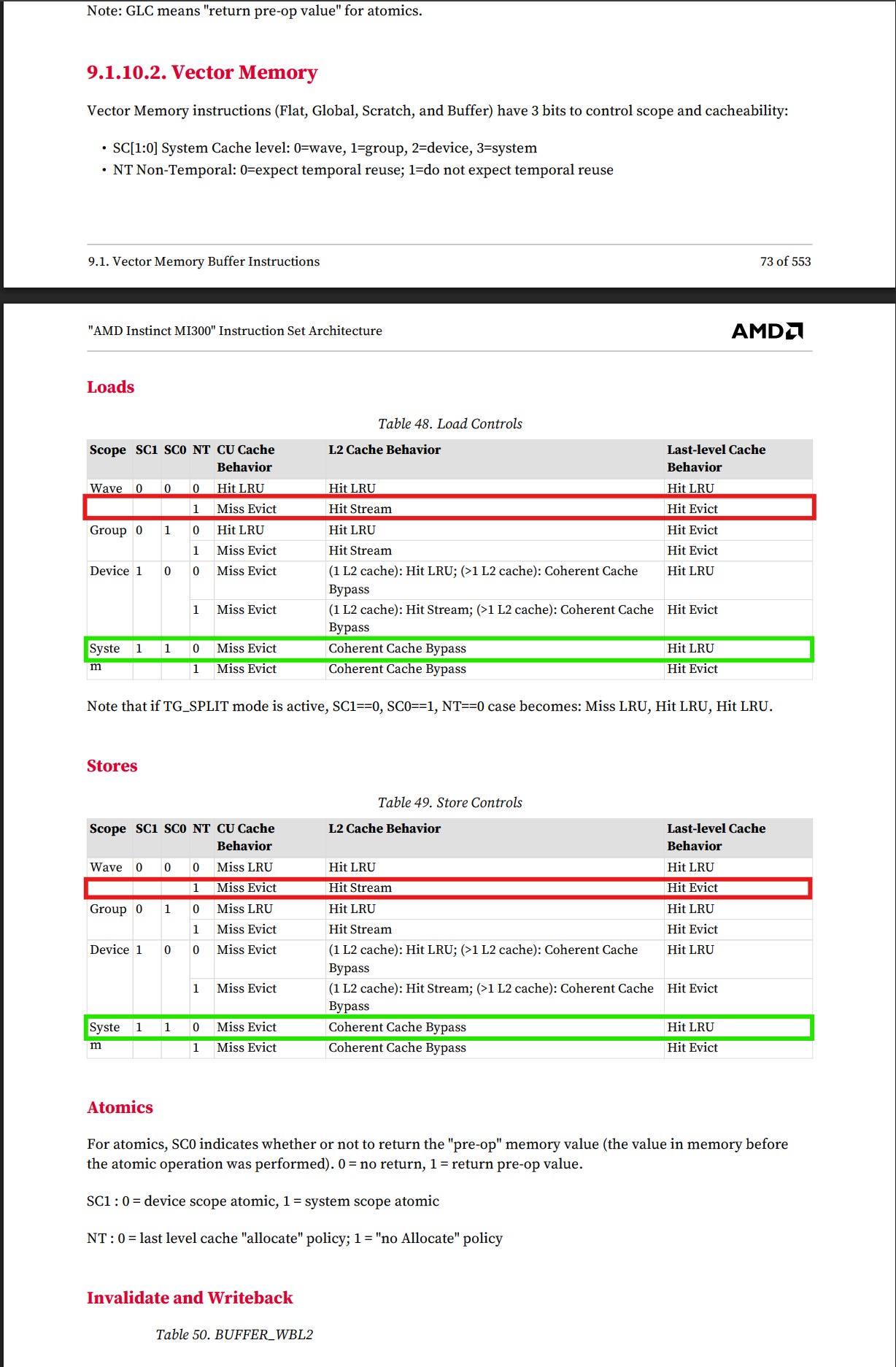
Here’s an image from the AMD documentation on how we can control loads and stores within our GPUs with respect to the memory hierarchy we described earlier. Some points to keep in mind here:
SC1 and SC0 are scope control bits, which control the “privateness” of the data at each level — SC0 for L1 cache, and SC1 for the L2.
Together with the NT bit, which is user specified, the L1 and L2 cache policies is determined.
For those curious, I confirmed with some people affiliated with AMD that no, we cannot bypass the L1C in a similar fashion. So, we wish to bypass the L2 as we have zero temporal locality. Let’s do that. Here’s the optimized kernel:
__device__ __forceinline__ float load_cache_bypass_dword(const float* ptr) {
    return __hip_atomic_load(ptr, __ATOMIC_RELAXED, __HIP_MEMORY_SCOPE_SYSTEM);
}

__device__ __forceinline__ void store_cache_bypass_dword(float* ptr, float val) {
    __hip_atomic_store(ptr, val, __ATOMIC_RELAXED, __HIP_MEMORY_SCOPE_SYSTEM);
}

__global__ void vectorAdd(const float* A, const float* B, float* C, int n) {
    int idx = blockIdx.x * blockDim.x + threadIdx.x;
    if (idx < n)
        store_cache_bypass_dword(C + idx, load_cache_bypass_dword(A + idx) + load_cache_bypass_dword(B + idx));
}
Notice how we use the __hip_atomic_load and hip_atomic_store intrinsics. We set the scope as per the table to bypass the L2. And __ATOMIC_RELAXED just tells the load to avoid using strict atomic rules, which would mean that our loads would enter the memory system one after another rather than in parallel.
How does performance change?
Now, let’s look at post-optimization perf counter results. First, a sanity check to make sure that the L2C hit rate dropped to zero post-bypass.
================================================================================
  L2 CACHE (TCC) ANALYSIS
================================================================================

L2 Cache Hit Rates:
  Hit Rate (reported):.........................    0.07%
  Hit Rate (calculated):........................   0.07%
  Cache Hits:................................... 3112
  Cache Misses:................................. 4194736
  Total Accesses:............................... 4197848

L2 Cache Traffic:
  Read Requests:................................ 2100696
  Write Requests:............................... 2097152
  Atomic Requests:.............................. 0

L2 Request Types by Caching Mode:
  Non-Coherent (NC):............................ 0
  Uncached (UC):................................ 314
  Coherent Cached (CC):......................... 0
  Read-Write (RW):.............................. 0

L2 Cache Evictions:
  Writebacks to DRAM:........................... 2097272
  Cache Line Evictions:......................... 1973462

L2 EA Uncached Traffic:
  Uncached Reads  (32B):........................ 630
  Uncached Writes (32B):........................ 2097152

L2 Tag Pipeline Activity:
  Total Tag Block Requests (TCC_REQ):........... 4197819
  Streaming Requests:........................... 0
  Tag Pipeline Stall:...........................   4.87%
  Tag Stall Cycles:............................. 1323206
  Tag RAM Stall Rate:...........................   0.00%

L2 Eviction & Writeback Breakdown:
  Normal Evictions (cache pressure):............ 1973462
  Invalidate-triggered Evictions:............... 0
  Normal Writebacks (dirty evictions):.......... 0
  TC_OP Writeback Requests:..................... 0

L2 Tag Overhead Analysis:
  Tag requests vs cache accesses delta:.........  -0.00%
Looks like the hit rate did indeed drop to zero as we’d expect post-cache bypass. Additionally, seems like the write-back that come when a cache line needs to be evicted have now flatlined, along with a lower tag pipeline stall rate, as we no longer compute tags for data going through the kernel. Correspondingly, tag stall cycles have also been halved. With lower cache traffic from L2 in general, it seems like the code to bypass is indeed functioning as one would image.
But what about the actual ramifications for perf? Let’s look at the average memory access latency:
 Memory Controller (EA) Status:
  EA Utilization:...............................      93.04%
  Write Starve Rate:............................       0.00%

Memory Latency:
  Average Read Latency (EA):....................    1033.90 cycles
Traffic going off the XCD has dropped a bit, and the best part is that the trip to memory has been shorted. So there appear to be improvements. Or so we think.
Achieved Bandwidth:
  From FETCH/WRITE_SIZE:........................    4383.01 GB/s
  Peak HBM Bandwidth (MI300X):             5300 GB/s
  Bandwidth Efficiency:.........................      82.70%
And the roofline.
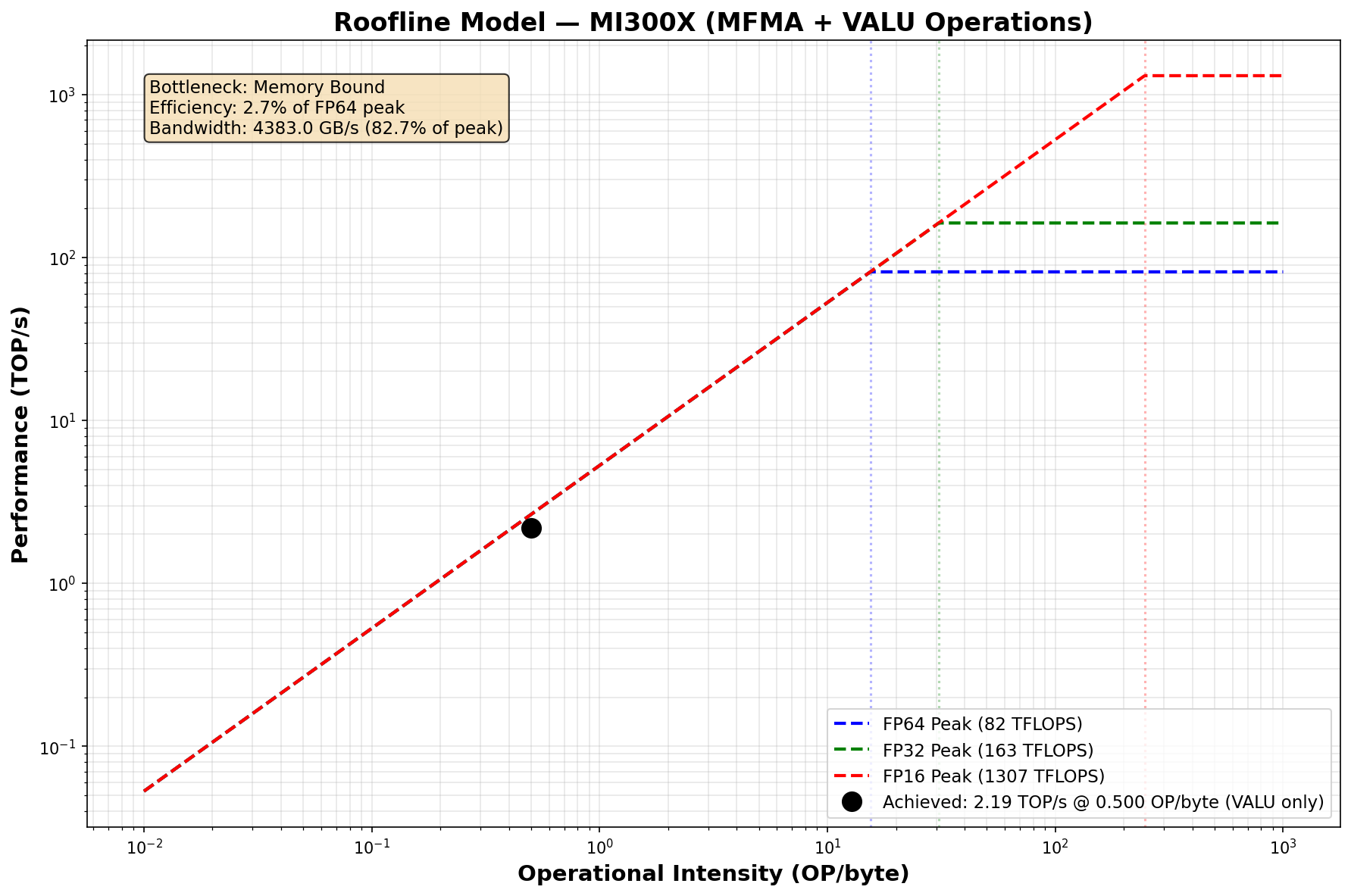
Wow, our bandwidth util jumped up quite a bit! Good to see. I will caution taking this result with a heavy bit of salt as the numbers here do very +/- 7% for the baseline and optimized version, so this may as well have been “cherry picked”. But understanding spatio-temporal loads, and whether you can disable redundant mechanisms in the memory hierarchy serves as a great starting point to data-driven runtime speedups in memory bound kernels. These are critical for certain decode generation kernels. The most common - and honestly really cliche - example of a kernel facing this problem are scaled-dot-product attention kernels.
Caveats on Data Collection That I faced
Currently, it doesn’t appear that we can fully track both EA port metrics. We can only gather data for EA0, one of the ports to InfinityCache. That generally means certain metrics may be impacted, namely the following in the data that I share:
Average Read Latency (EA)
Total Read Requests to DRAM (underreported)
Total Write Requests to DRAM (underreported)
Total DRAM Traffic
Estimated Read/Write DRAM Volume
Conclusion
In this blog, we walked through an optimization that speeds up the vector add workload, which is inherently memory bound. We demonstrate better bandwidth utilization in a non “hand-wavy” way, one grounded in data that we can observe and analyze.
Most performance engineering optimizations can be speculated on their value purely through a back-of-the-envelope calculation on arithmetic intensity. However, without a fundamentally data-driven approach to understanding what our workloads end doing, performance engineering remain “a grab bag of tricks” that we purely chuck at the wall to see what sticks. Practically speaking however, leveraging performance counter data effectively is hard — in a standard Megatron-LM / Deepspeed pre-training or inference, thousands of kernels are launched, making it nearly impossible to gather data tractably (in a reasonable amount of time) with such fine grained methods.
The Code
Codebase is here: https://github.com/AnshKetchum/kernel-profiling-hip
The actual document with the final stats for optimized results are here
The baseline is here.
Being upfront here that some of my numbers reported are outdated from the final values pushed. Take results with a grain of salt.
Follow the instructions on the README, hopefully they’re clear enough. If not, feel free to contribute or reach out! I generally respond pretty quickly to these messages.
References
https://www.amd.com/en/products/accelerators/instinct/mi300/mi300x.html
https://hc2024.hotchips.org/assets/program/conference/day1/23_HC2024.AMD.MI300X.ASmith(MI300X).v1.Final.20240817.pdf
https://computermachines.org/joe/publications/pdfs/isca2024_exascale.pdf
https://llvm.org/docs/AMDGPUUsage.html#memory-model-gfx942
https://www.amd.com/content/dam/amd/en/documents/instinct-tech-docs/instruction-set-architectures/amd-instinct-mi300-cdna3-instruction-set-architecture.pdf
https://github.com/Dao-AILab/flash-attention
Appendix
** I explicitly refer to the data as “bytes of data” and not just “all the data” because caches track some comparably tiny but non-trivial amounts of metadata as well, meaning the data transfer itself is a bit larger.
Questions I haven’t gotten a chance to answer
Why is the L2 Read Traffic the same as the write traffic?
Feel free to add to this list!! It can get pretty lonely solo-blogging, reach out if you have any Q’s! :D
Corrections
This blog is by all means, incorrect in some areas. It was pretty hastily written, so if you have any feedback or pointers on inconsistencies, please send them my way. I’ll list the ones suggested here below as they arrive.